L1-python/source/Plotting1.ipynb

Libraries

# libraries
import scipy 
# "SciPy" provides algorithms for optimization, integration, interpolation, eigenvalue problems, 
# algebraic equations, differential equations, statistics and many other classes of problems.
import numpy as np
# Fast and versatile, the "NumPy" vectorization, indexing, and broadcasting concepts are the 
# de-facto standards of array computing today.
import matplotlib.pyplot as plt
# "Matplotlib" is a comprehensive library for creating static, animated, and interactive 
# visualizations in Python.

Data

x= np.linspace(0,2*np.pi)
y= np.sin(x)

Anatomy of a figure

%matplotlib inline
from PIL import Image
img = Image.open('anatomy.webp')
img.save("anatomy.png")

# import image module
from IPython.display import Image
  
# get the image
Image(url="anatomy.png", width=500, height=500)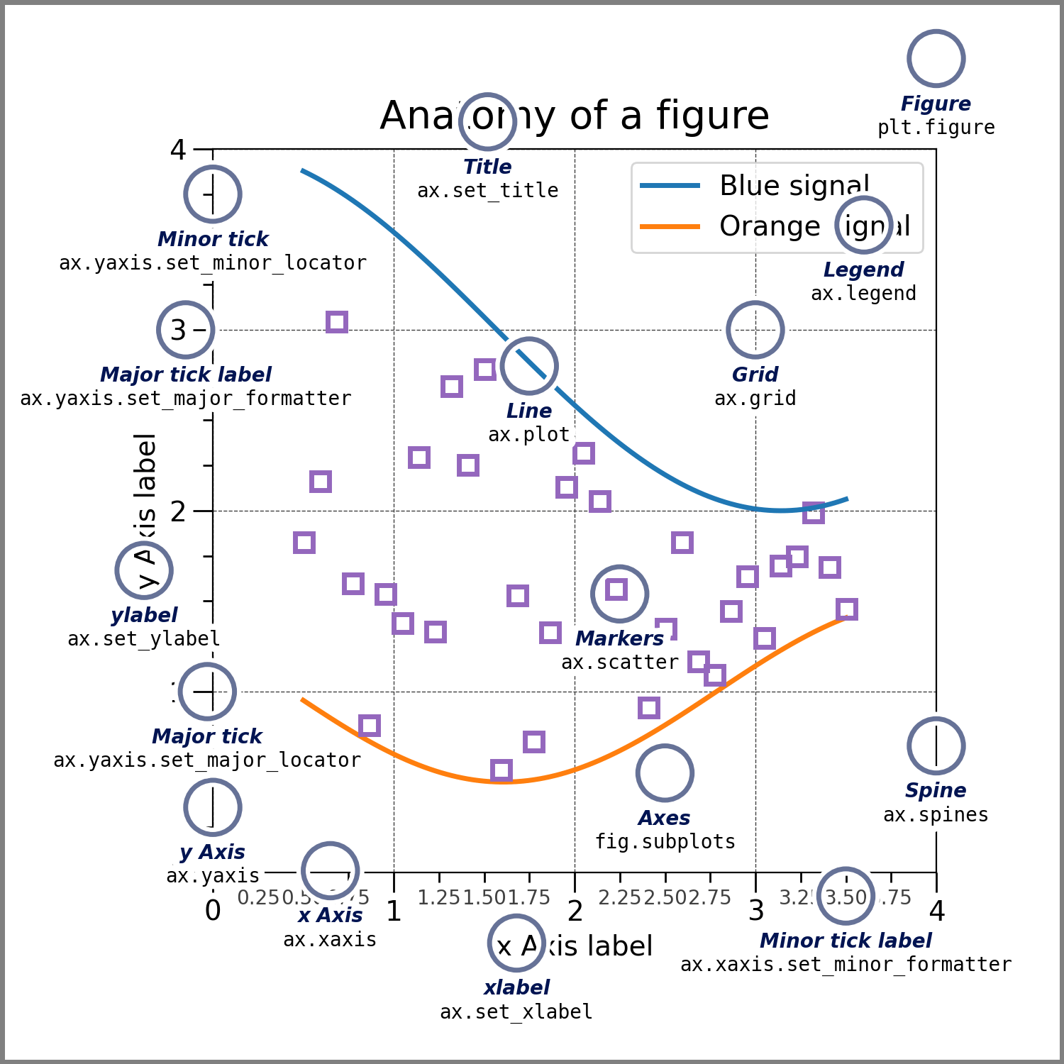

Implicit or explicit?

Using figures

• Explicitly create Figures and Axes, and call methods on them (the "object-oriented (OO) style").
• Rely on pyplot to implicitly create and manage the Figures and Axes, and use pyplot functions for plotting.

# implicit 
plt.plot(x,y,label="sin")
plt.xlabel('x label')
plt.ylabel('y label')
plt.title("Simple Plot")
plt.legend()
plt.show()

# explicity
fig = plt.figure(figsize=(6,6)) # size
ax = plt.subplot(aspect=1)   # aspect ratio
ax.plot(x,y,label="sin") # label
ax.set_xlabel('x')  # Add an x-label to the axes.
ax.set_ylabel('y')  # Add a y-label to the axes.
ax.set_title("Simple Plot")  # Add a title to the axes.
ax.legend() # Add a legend.

<matplotlib.legend.Legend at 0x7fcca3b14dc0>

Figure : lines

fig = plt.figure(figsize=(6,6))
ax = plt.subplot(aspect=1)
ax.plot(x,y,label="sin",color='blue', linewidth=3, linestyle='--') 
ax.plot(x,y*y,label="$\sin^2$",color='red', linewidth=1, linestyle='dotted') 
ax.set_xlabel('x')  # Add an x-label to the axes.
ax.set_ylabel('y')  # Add a y-label to the axes.
ax.set_title("Simple Plot")  # Add a title to the axes.
ax.legend() # Add a legend.

<matplotlib.legend.Legend at 0x7fdc69fe4b90>

ax.plot?

Figure and Axes

#
fig = plt.figure(figsize=(6,6))
ax = plt.subplot(aspect=1)
ax.plot(x,y,".r",label="$\sin(x)$") 
ax.plot(x,y*y,".g",label="$\sin(x)^2$") 
ax.legend()
ax.set_xlabel("x")
ax.set_ylabel("y")

Text(0,0.5,'y')

Figures : axes and text

# adding text
fig = plt.figure(figsize=(6,6))
ax = plt.subplot(aspect=1)
ax.plot(x,y,".",label="sin") 
ax.legend()


ax.text(0.3,  0.1, "-> Mot",family="cursive",size=14)
ax.text(0.3, -0.5, "-> Mot",family="serif",size = 14)

ax.annotate('point (3,0)', xy=(3, 0), xytext=(4, 0.5),
            arrowprops=dict(facecolor='black', shrink=0.05))

ax.set_title('Title')
ax.set_xlabel("x")
ax.set_ylabel("y")

Text(0,0.5,'y')

figure : scales

fig = plt.figure(figsize=(6,6)) # size
ax = plt.subplot(aspect=1)   # aspect ratio

ax.plot(x,y,label="sin") # label
ax.set_xscale('log')
ax.set_yscale('log')
ax.set_xlabel('x')  # Add an x-label to the axes.
ax.set_ylabel('y')  # Add a y-label to the axes.
ax.set_title("Title")  # Add a title to the axes.
ax.legend() # Add a legend.

<matplotlib.legend.Legend at 0x7fdc5860e790>

figures multiples

fig, (ax0, ax1, ax2) = plt.subplots(nrows=1, ncols=3,
                                    figsize=(6, 6))
fig.tight_layout()
ax0.set_title('a')
ax0.plot(x,y,label="sin") # label

ax1.plot(x,y,label="sin") # label

ax2.set_title('title')
ax2.plot(x,y,label="sin") # label

[<matplotlib.lines.Line2D at 0x7fdc69e73190>]

figure : save

#save
fig.savefig("output.png")
fig.savefig("output.pdf")